Using NESTA-NMR¶
Location of sample scripts¶
All of the scripts described in this manual can be found in the scripts
directory of NESTA-NMR.
Conversion to NMRPipe format¶
As of version 1.5, NESTA-NMR contains changes to the way data are prepared prior to reconstruction by NESTA-NMR. Instead of converting the data in its sparse format, it is now expanded to its final (reconstructed) size with the unsampled data points being filled with zeros. These changes will require adjustment to the initial conversion steps, but has the advantage of making data processing more like that of regular (uniformly sampled) data. Importantly, these changes will also help ensure compatibility with on-going improvements to the ability of NMRPipe [*] to handle NUS data. This procedure is described below in the section on expanded data conversion.
The old method (see sparse data conversion) is still supported by the current version of NESTA-NMR and is necessary in the case of very large data sets (e.g. 4D spectra with high resolution in all indirect dimensions) until NMRPipe is fully 64-bit (see issues with 32-bit software). However, all other data conversions should be performed using the new method. Future versions of NESTA-NMR will no longer accept sparse data.
Because the data are now converted to full size before running
bruk2pipe or var2pipe, the conversion can be performed exactly
as it would be for uniformly sampled data. This means the dimension
sizes (-yN and -yT, -zN and -zT, and -aN and
-aT) correspond to their final sizes and the quadrature modes
(-yMODE, -zMODE, and -aMODE) can be correctly set to
Rance-Kay, States, States-TPPI, etc. For this reason, the NMRPipe
Rance-Kay macros (NESTA_bruk_ranceN.M and NESTA_var_ranceN.M)
that were previously used with sparse data (see the Rance-Kay section) are
no longer required. Additionally, the NESTA-NMR flag for sign
alternation (–alt, see the section on NESTA-NMR setup) is no longer needed
since States-TPPI can be set during conversion.
Expanded data conversion (new style)¶
Conversion of Bruker and Varian/Agilent data to NMRPipe format now has two steps:
- Expand data into a zero-filled matrix using the NMRPipe program
nusExpand.tcl - Convert data to NMRPipe format using
bruk2pipeorvar2pipe
These two functions can be handled by running the respective GUI
conversion commands with a -nus flag: bruker -nus or
varian -nus. Setting the correct “Dimension Count” (see the image of
Bruker 2D conversion) on the top right section and then pressing “Read
Parameters” seems to do an excellent job of interpreting the data and
NUS settings.
Note that bruker -nus and varian -nus create a sample setup for
the two conversion steps above, as well as an additional, second call to
nusExpand.tcl (see bottom of the Conversion Script Text window
in the image below). This last call to nusExpand.tcl
produces a mask that is not needed by NESTA-NMR, so it can be removed
from the script before execution. In the case of very large file sizes,
this third command will produce errors and should definitely be removed.
For all of the included sample scripts, this command has been deleted.
Examples are shown for 2D Bruker, 3D Varian/Agilent, and 4D Bruker data below. Important aspects of the conversion are noted.
The details of nusExpand.tcl are described in the section on data expansion.
For bruk2pipe, the final size of the data in the indirect dimension
is used for -yN and -yT, and -yMODE is now set to the
correct quadrature method, which is Rance-Kay here.
A version of this script, called fid_2D.com, which omits a few
unnecessary flags, removes the second nusExpand.tcl command, and
also optionally deletes expanded files once they are no longer needed,
can be found in the scripts directory.
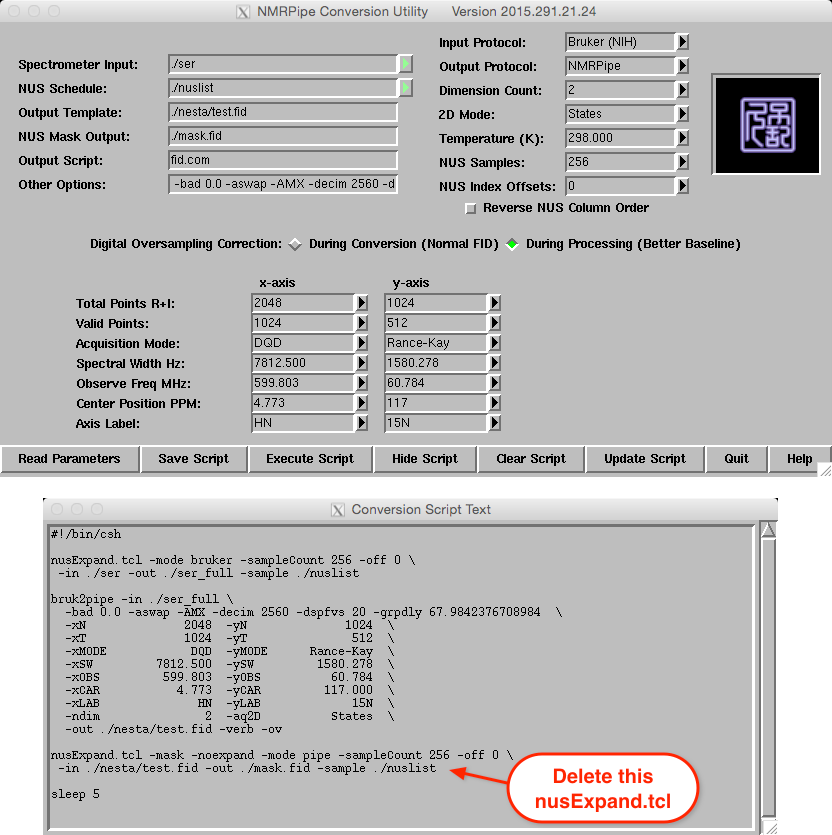
Conversion from Bruker to NMRPipe for 2D data.
Conversion of a 3D Varian/Agilent data set is shown below. Again, note
that final (expanded) sizes are entered for the Y- and Z-dimensions and
the correct quadrature protocols are used. This particular
Varian/Agilent data set was collected with the acquisition order set to
phase,phase2 in the procpar, which is denoted by the
-aqORD 1 flag in the var2pipe command. See the section on Varian/Agilent processing for
more details.
A version of this script, called fid_3D.com can be found in the scripts directory.
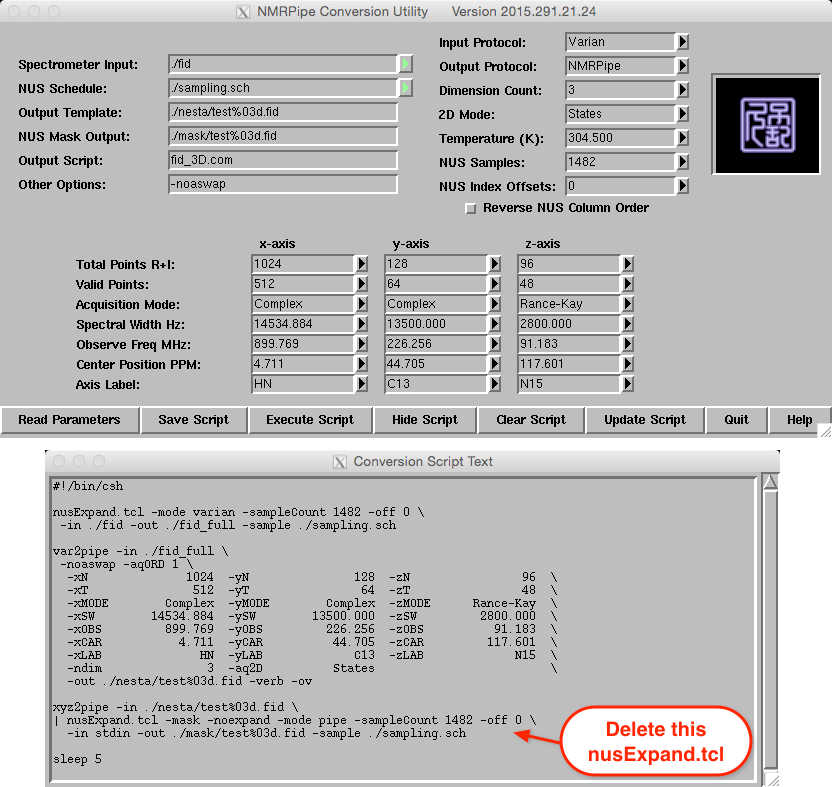
Conversion from Varian/Agilent to NMRPipe for 3D data.
Conversion of a 4D Bruker data set is shown below. As with the 2D and 3D
data, note the use of final expanded dimension sizes for the Y-, Z-, and
A-axes and use of States-TPPI for quadrature. As noted in the sections on
data conversion and NESTA-NMR setup, the NESTA-NMR –alt flag for
States-TPPI sign alternation is now deprecated since this can be set
directly during conversion.
A version of this script, called fid_4D.com can be found in the scripts directory.
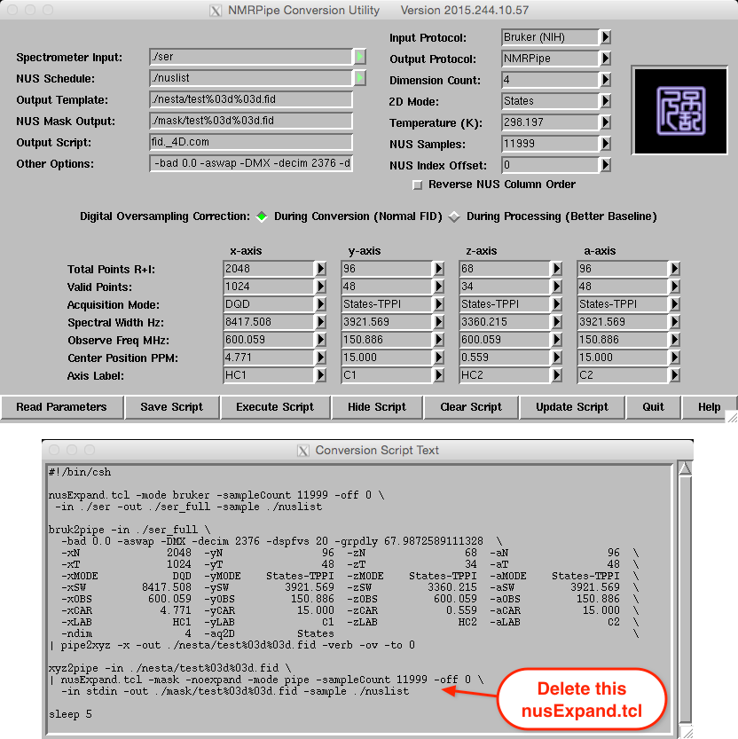
Conversion from Bruker to NMRPipe for 4D data.
Acquisition order for expanded Varian/Agilent data¶
Varian/Agilent spectrometers allow the acquisition order to be set for
experiments that have more than one indirect dimension, i.e. 3D or 4D.
NESTA-NMR expects data that are acquired with an acquisition order of
phase2,phase and phase3,phase2,phase for 3D and 4D data,
respectively, in the procpar file.
For Varian/Agilent data that were collected using an alternative
acquisition order, the adjustment should be made during var2pipe
with the -aqORD flag in
var2pipe,
see the Varian/Agilent conversion figure. Previously, it was recommended that this
be done with varAdjust.tcl, but this is no longer the recommended
method.
Sparse data conversion (old style)¶
This method of data conversion is deprecated, as noted in the section on data conversion. To ease the transition and to enable the processing of very large spectra (see the section on 32-bit program issues) until NMRPipe is fully 64-bit, it will remain in NESTA-NMR for version 1.5, with a few minor changes being required to maintain compatibility with recent versions of NMRPipe. The required changes are noted in this section.
Because the sparse conversion method is only required for large data, the following instructions will primarily cover the conversion of 4D spectra.
Acquisition order for sparse Varian/Agilent data¶
Adjustment of Varian/Agilent acquisition order was previously
accomplished with the NMRPipe function varAdjust.tcl, however the
current recommendation is to use the -aqORD flag in var2pipe, as
is discussed in the section on Varian/Agilent processing.
Conversion of sparse data to NMRPipe format¶
Due to the sparsity of unexpanded NUS data, several adjustments must be employed when converting data into a format readable by NMRPipe. During data acquisition, it is particularly important to note the spectral widths and offset positions for the indirect dimensions as these values are sometimes not correctly detected.
For example, for 4D sparse data, the quadrature method, -yMODE,
-zMODE, and -aMODE, must always be set to Real. For the
Y-dimension, the total number of points, -yN, and the time domain
size, -yT, must be set to 8 (2N, where N is the
number of NUS dimensions). The number of points in the second indirect
dimension (-zN and -zT) must correspond to the number of NUS
points.
There are also a couple of changes required specifically for data
processed with recent versions of NMRPipe [†], due to alterations in
the way it handles data conversion. If the spectrum is a 4D, the number
of points in the A-dimension (-aN and -aT) must both be set to
0, not 1 as was done with previous versions of NESTA-NMR. Finally,
for a 4D spectrum, the number of dimensions, -ndim must be set to
3, not 4 as was done with previous versions of NESTA-NMR. For sparse
2D and 4D data, no additional changes need to be made during conversion.
The script fid_4D_sparse.com demonstrates all of these changes for
conversion of a 4D data set. It is important to ensure that the output
template, which is test%05d.fid here, contains only one template
position (i.e. %05d) for sparse data and has enough decimal places
to accommodate the number of NUS points.
#!/bin/tcsh

# Conversion of 4D NUS experiment to NMRPipe format for NESTA-NMR

# NOTE: This script is only for sparse data. Please transition to
#       using the expanded data conversion method as the sparse
#       method will soon not be supported by NESTA-NMR.

bruk2pipe -in ./ser \
-bad 0.0 -aswap -DMX -decim 2376 -dspfvs 20 -grpdly 67.9872589111328  \
-xN        2048  -yN            8  -zN        12000  -aN           0  \
-xT        1024  -yT            8  -zT        12000  -aT           0  \
-xMODE      DQD  -yMODE      Real  -zMODE      Real  -aMODE     Real  \
-xSW   8417.508  -ySW    3921.569  -zSW    3360.215  -aSW   3921.569  \
-xOBS   600.059  -yOBS    150.886  -zOBS    600.059  -aOBS   150.886  \
-xCAR     4.771  -yCAR     15.000  -zCAR      0.559  -aCAR    15.000  \
-xLAB       HC1  -yLAB         C1  -zLAB        HC2  -aLAB        C2  \
-ndim         3  -aq2D     States                                     \
-out ./nesta/test%05d.fid -verb -ov
Process direct dimension¶
Expanded data¶
After conversion to NMRPipe format, the directly detected dimension is
processed as usual, including solvent suppression, apodization,
zero-filling, Fourier transformation, and phasing. The number of
reconstructions performed by NESTA-NMR is dictated by the number of
directly detected points, so it is best to extract only the relevant
region using the NMRPipe extract (EXT) function before saving the
slices. Additionally, it is desirable to remove any solvent and buffer
signal, either through extraction or solvent suppression techniques, as
NESTA-NMR will reconstruct these signals.
An example script, , that extracts the methyl region of the directly detected dimension from a 4D experiment is shown. NESTA-NMR expects data whose axes are in the same order as they were acquired, so it is important not to transpose the data before reconstruction.
#!/bin/tcsh

# Processing of the direct dimension of a 4D for NESTA-NMR

xyz2pipe -in ./nesta/test%03d%03d.fid -verb -x         \
| nmrPipe  -fn SOL                                 \
| nmrPipe  -fn SP -off 0.5 -end 0.98 -pow 1 -c 0.5 \
| nmrPipe  -fn ZF -auto                            \
| nmrPipe  -fn FT -auto                            \
| nmrPipe  -fn PS -p0 0.0 -p1 0.0 -di              \
| nmrPipe  -fn EXT -x1 1.5ppm -xn -1ppm -sw        \
| pipe2xyz -out ./nesta/test%03d%03d.dat -x
It is recommended that the suffix dat be used for un-reconstructed
data that has been processed in the direct dimension. This helps to
avoid confusion (and the accidental overwriting of files) as NESTA-NMR
uses the suffix ft1 for reconstructed data.
Sparse data¶
The section on direct dimension processing of expanded describes how to process the direct dimension of
expanded data. As long as the Rance-Kay protocol was not used for
any of the indirect dimensions, this same conversion script
(nmrproc_direct.com) can be used for sparse data. The only
adjustment that may need to be made is the template name for input and
output filenames. In particular, as can be seen in the output command of
the file fid_4D_sparse.com, the conversion of 4D sparse data
requires only a single dimension in the template format.
Sparse data with Rance-Kay acquisition¶
For sparse data, if any of the indirectly detected dimensions utilize
the Rance-Kay (also called Echo-AntiEcho) protocol for frequency
discrimination, an additional step is required during processing of the
direct dimension. This step utilizes one of two NMRPipe macros, either
NESTA_bruk_ranceN.M or NESTA_var_ranceN.M for Bruker and
Varian/Agilent, respectively, which are found in the NMRPipe
directory of NESTA-NMR.
The dimension requiring Rance-Kay processing is set within the NMRPipe
macro function call using the variable nShuf. If the first indirect
dimension (Y) requires Rance-Kay processing, the value for nShuf is
1 (see example below). For the second (Z) and third (A) indirect
dimensions the values of nShuf are 2 and 3, respectively. Only one
value can be entered for nShuf, so the presence of multiple
Rance-Kay detected dimensions would require additional calls to the
macro command.
The following script, , is an example that utilizes NESTA_ranceN.M
for the Rance-Kay protocol for the Y- and Z-axes. The path to the macro
can be provided with a shell variable, as is demonstrated with
NESTAMACRO.
#!/bin/tcsh

# Processing of the direct dimension of a 3D/4D for NESTA-NMR
# With Rance-Kay acquisition in first (Y) and second (Z) dimensions

# NOTE: This script is only for sparse data where the Rance-Kay protocol
#       has to be performed during processing of the direct dimension.
#       Please transition to using the expanded data conversion method
#       as the sparse method will soon not be supported by NESTA-NMR.

setenv NESTAMACRO $HOME/local/NESTANMR/NMRPipe

xyz2pipe -in ./nesta/test%05d.fid -verb -x                                   \
| nmrPipe -fn MAC -macro $NESTAMACRO/NESTA_bruk_ranceN.M -noRd -noWr -var nShuf 1 \
| nmrPipe -fn MAC -macro $NESTAMACRO/NESTA_bruk_ranceN.M -noRd -noWr -var nShuf 2 \
| nmrPipe  -fn SOL                                                           \
| nmrPipe  -fn SP -off 0.5 -end 0.98 -pow 1 -c 0.5                           \
| nmrPipe  -fn ZF -auto                                                      \
| nmrPipe  -fn FT -auto                                                      \
| nmrPipe  -fn PS -p0 0.0 -p1 0.0 -di                                        \
| nmrPipe  -fn EXT -x1 1.5ppm -xn -1ppm -sw                                  \
| pipe2xyz -out ./nesta/test%05d.dat -x
Correction for States-TPPI frequency discrimination with sparse data
requires the use of sign alternation during Fourier transform of the
appropriate dimension (see the section on general processing). This can either be specified
through the use of a header flag that is set during reconstruction (see the
section on NESTA-NMR setup) or by a flag used with the NMRPipe function FT
(see the processing section). Details are provided where appropriate. No
additional commands or flags are required for States frequency
discrimination.
Reconstruct missing data¶
NESTA-NMR is designed to reconstruct 2D, 3D, and 4D data with a single command. The program attempts to detect the correct settings where possible, but its default behavior can be modified through a series of command line flags.
Quickstart¶
In most cases, NESTA-NMR can be executed with a single command (or shell script), which requires only the file template as an input, as demonstrated by:
#!/bin/tcsh

# Basic execution of NESTA-NMR

$HOME/local/NESTANMR/binaries/NESTANMR -f ./nesta/test%03d%03d.dat
The defaults for NESTA-NMR are designed to produce excellent results. However, there are many options to customize the performance and output of NESTA-NMR, as described below.
NESTA-NMR execution with sparse data¶
One additional change must be made to NESTA-NMR when reconstructing
sparse data: the flag -u or –unexpanded must be added to the
NESTA-NMR command line. See the NESTA-NMR setup section.
Setup NESTA-NMR¶
The input options are described in more detail below, but they can be
summarized from the command line by typing NESTANMR -h or
NESTANMR –help. The flags listed are described in the reference for
NESTA-NMR command line output. The meaning of each flag is
explained further in the command reference.
Run NESTA-NMR¶
NESTA-NMR is run by calling the program with the appropriate set of flags, as described above. A simple example might need to specify only the input template and the number of cores:
#!/bin/tcsh

# Basic execution of NESTA-NMR with threads set

$HOME/local/NESTANMR/binaries/NESTANMR -f ./nesta/test%03d%03d.dat -t 16
Unless the –quiet flag is used (see the NESTA-NMR setup section), NESTA-NMR
prints a progress message similar to this to indicate its progress
through points in the direct dimension:
************************************************************************************
*                                   NESTA-NMR v1.5                                 *
*     Shangjin Sun, Michelle Gill, Yifei Li, Mitchell Huang, and R. Andrew Byrd    *
*                         Structural Biophysics Laboratory                         *
*                            National Cancer Institute                             *
*                               Frederick, MD 21702                                *
*                                                                                  *
*              Use of NESTA-NMR implies acceptance of the user license             *
************************************************************************************

******** SETTINGS ********
fids = ./nesta/test
nuslist = ./nuslist
outdir = nesta
outname = test
threads = 12
method = 1
iter = 30
quiet = 0
keepnesta = 0
sparse = 0

Begin NESTA-NMR slice:    7
Begin NESTA-NMR slice:   11
Begin NESTA-NMR slice:    9
Begin NESTA-NMR slice:    3
Begin NESTA-NMR slice:    5
Begin NESTA-NMR slice:    2
Begin NESTA-NMR slice:   10
Begin NESTA-NMR slice:    6
Begin NESTA-NMR slice:   12
Begin NESTA-NMR slice:    8
Begin NESTA-NMR slice:    4
Begin NESTA-NMR slice:    1
End NESTA-NMR slice    9. Slice run time is 42 second(s).
End NESTA-NMR slice   10. Slice run time is 42 second(s).
End NESTA-NMR slice    7. Slice run time is 42 second(s).
End NESTA-NMR slice    5. Slice run time is 42 second(s).
End NESTA-NMR slice    4. Slice run time is 42 second(s).
End NESTA-NMR slice    2. Slice run time is 42 second(s).
End NESTA-NMR slice    3. Slice run time is 42 second(s).
End NESTA-NMR slice    1. Slice run time is 42 second(s).
End NESTA-NMR slice    8. Slice run time is 42 second(s).
End NESTA-NMR slice   12. Slice run time is 42 second(s).
End NESTA-NMR slice    6. Slice run time is 42 second(s).
End NESTA-NMR slice   11. Slice run time is 42 second(s).
...
For 2D spectra, messages are not printed for individual slices (directly detected points). If multi-threaded processing is used and slice number are printed, they may appear out of order, as shown above. This is due to the way the multiprocessing library works and does not affect the final output.
Processing 2D spectra with NESTA-NMR L1 takes less than about a minute. For 3D spectra, typical processing times are 1-5 minutes. For 4D spectra, processing can take between 30 minutes and approximately three hours, with 30 iterations of \(\mu\), depending on the number of points in the direct dimension and hardware capabilities.
Output files¶
NESTA-NMR creates output files that use outname as a base and
ft1 as an extension. The files are stored in the directory set by
the flat outdir. For 2D reconstructions, only a single file is
created, e.g. test.ft1. For reconstruction of 3D and 4D expanded
data, NESTA-NMR uses the same template scheme as the input data. For
sparse data, 3D reconstruction files are created using a template with
four decimal places (%04d), e.g. test0001.ft1. For sparse 4D
reconstructions, the files use %03d%03d, e.g. test001001.ft1.
If the –keepnesta flag was set during reconstruction, the temporary
input and output files that NESTA-NMR uses for file reconstruction will
also be preserved. These files use the flag –outname for a base and
have nestain and nestaout extensions, respectively. They are
stored in the directory specified by the flag –outdir. The primary
use of these files is for debugging.
Log files can be used to evaluate the success of the reconstruction, as described in the next section.
Evaluate reconstruction¶
NESTA-NMR creates a log file for each slice during reconstruction. These
files use the outname as a base and are stored in outdir with a
log extension: ./nesta/test0001.log, ./nesta/test0002.log,
etc. These files can be used to determine the reconstruction success of
each of the slices. The value of greatest importance is the very last
value for fx_diff in each of the files. This is a measure of the
error in the final reconstructed data slice relative to the initial
data. Typical values for L1 reconstruction are in the \(10^{-13} - 10^{-11}\)
range, while IRL1 values are of
order \(10^{-5}\) due to the effect of re-weighting on the
error value. For Gaussian-SL0, the convergence is evaluated based on the
set value of the cutoff relative to the final threshold reached.
A simple python script, called can be used to extract the error
(fx_diff) in the case of L1 and IRL1, or the steps to convergence
and threshold value, in the case of Gaussian-SL0, from each of the log
files. A tab-delimited file, called , is created with these values. The
python script is not shown due to its length, but it is located in the
directory.
For L1 data, the file for a 4D reconstruction resembles this:
file         plane   fx(L1-norm)       fx_diff    time(s)
test0001.log     1    3.5060e+11    6.7944e-11         41
test0002.log     2    2.8398e+11    8.5588e-11         39
test0003.log     3    2.4323e+11    9.9352e-11         36
...
test0246.log   246    2.2280e+11    1.0821e-10         38
test0247.log   247    2.7450e+11    8.6175e-11         40
test0248.log   248    3.3746e+11    7.3660e-11         42

Total computation time: 425 seconds
Elapsed (clock) time: 42 seconds
Parallelization speed up (comp time/elapsed time): 10.1 times
The file lists the log file, reconstruction plane, convergence value
(fx), error at convergence (fx_diff), and optimization time.
Optimization time should be considered an estimate because the precision
on the calculation is seconds. For 2D reconstructions, it is common for
the elapsed time for a single plane to be 0 seconds due to computational
precision of the command used for timing.
For IRL1 reconstruction, the file is similar except that error values
(fx_diff) may be different, as mentioned above.
For Gaussian-SL0 reconstruction, the file contains the log file, plane,
and reconstruction time, as is done for L1/IRL1 reconstructions.
However, instead of error (fx_dff), the number of iterations to
convergence and the threshold at convergence are shown.
Process indirect dimensions¶
After reconstruction is complete, the indirect dimensions of the data need to be processed. This is directly analogous to the treatment of uniformly sampled multidimensional data.
For sparse data (see the sparse data conversion section) only: if any of the reconstructed
dimensions utilized States-TPPI and the appropriate flag(s), e.g.
–alt yza for sign-alternation in all three dimensions, were set
during NESTA-NMR reconstruction, then the Fourier transform of that
dimension will automatically perform sign alternation as long as the
-auto flag is used, i.e. nmrPipe -fn FT -auto. If the flag was
not set when calling NESTA-NMR, sign alternation can be forced by use of
the -alt flag, i.e. nmrPipe -fn FT -alt.
Phasing 3D and 4D data from slices¶
If desired, the phases for the indirect dimensions can be determined
prior to processing the indirect dimensions. At the end of
reconstruction, NESTA-NMR creates slices in the output directory defined
by outdir. These slices are created as appropriate and are named
XY.ft1, XZ.ft1, and XA.ft1. They can then be processed with
the script .
#!/bin/tcsh

# This script processes the 2D slices created by NESTA-NMR
# These files are named XY.ft1, XZ.ft1, and XA.ft1
# and are created in the NESTA-NMR output directory ("nesta" here)
# If the slices have been deleted, they can be recreated with
# the script "nmrproc_make_slices.com" rather than having to
# re-run NESTA-NMR.


# The XY dimension
echo "Processing the XY slice..."

nmrPipe -in ./nesta/XY.ft1 -verb                  \
| nmrPipe -fn TP                                  \
| nmrPipe -fn SP -off 0.5 -end 0.95 -pow 1 -c 1.0 \
| nmrPipe -fn ZF -auto                            \
| nmrPipe -fn FT -auto                            \
| nmrPipe -fn PS -p0 0.0 -p1 0.0 -di              \
-out ./nesta/XY.ft2 -ov

# The XZ dimension for a 3D or 4D
echo "Processing the XZ slice..."

nmrPipe -in ./nesta/XZ.ft1 -verb                  \
| nmrPipe -fn TP                                  \
| nmrPipe -fn SP -off 0.5 -end 0.95 -pow 1 -c 1.0 \
| nmrPipe -fn ZF -auto                            \
| nmrPipe -fn FT -auto                            \
| nmrPipe -fn PS -p0 0.0 -p1 0.0 -di              \
-out ./nesta/XZ.ft2 -ov

# The XA dimension for a 4D
echo "Processing the XA slice..."

nmrPipe -in ./nesta/XA.ft1 -verb                  \
| nmrPipe -fn TP                                  \
| nmrPipe -fn SP -off 0.5 -end 0.95 -pow 1 -c 1.0 \
| nmrPipe -fn ZF -auto                            \
| nmrPipe -fn FT -auto                            \
| nmrPipe -fn PS -p0 0.0 -p1 0.0 -di              \
-out ./nesta/XA.ft2 -ov
If the 2D slices are inadvertently deleted, the easiest way to recreate them without running NESTA-NMR again is to use the script .
#!/bin/tcsh

# This script recreates the 2D slices originally
# created by NESTA-NMR. These files are named
# XY.ft1, XZ.ft1, and XA.ft1
# The template and test001001.ft1 file names
# may need to be adjusted as appropriate.


# The XY dimension
echo "Creating the XY slice..."

cp nesta/test001001.ft1 nesta/XY.ft1
sethdr nesta/XY.ft1 -ndim 2

# The XZ dimension for a 3D or 4D
echo "Creating the XZ slice..."

xyz2pipe -verb -in nesta/test%03d%03d.ft1 -z \
| pipe2xyz -out nesta/test%03d%03d.tmp -y -ov

cp nesta/test001001.tmp nesta/XZ.ft1
sethdr nesta/XZ.ft1 -ndim 2
rm nesta/*.tmp

# The XA dimension for a 4D
echo "Creating the XA slice..."

xyz2pipe -verb -in nesta/test%03d%03d.ft1 -a \
| pipe2xyz -out nesta/test%03d%03d.tmp -y -ov

cp nesta/test001001.tmp nesta/XA.ft1
sethdr nesta/XA.ft1 -ndim 2
rm nesta/*.tmp
An alternate method of creating and processing the slices that uses the
NMRPipe utilities ext.xz.com and ext.xa.com, which are located
in the NMRTXT directory of the NMRPipe program, is demonstrated in .
The variables XZ_slice and XA_slice can be used to select a
slice other than the first one for the respective dimension. The
variable NMRTXT is as defined by NMRpipe. Unfortunately, this method
sometimes fails to produce the correct slices and, thus, is not
recommended as a first choice.
#!/bin/tcsh

# This script uses the NMRPipe programs which extract data
# for the Z and A dimensions. Sometimes the programs don't
# extract data, thus this method isn't recommended.
# The template and test001001.ft1 file names
# may need to be adjusted as appropriate.

# The XY dimension
echo "Processing the XY slice..."

nmrPipe -in ./nesta/test001001.ft1 -verb          \
| nmrPipe -fn TP                                  \
| nmrPipe -fn SP -off 0.5 -end 0.95 -pow 1 -c 1.0 \
| nmrPipe -fn ZF -auto                            \
| nmrPipe -fn FT -auto                            \
| nmrPipe -fn PS -p0 0.0 -p1 0.0 -di              \
-out XY.ft2 -ov

# The XZ dimension for a 3D or 4D
echo "Processing the XZ slice..."

set XZ_slice=1
$NMRTXT/ext.xz.com ./nesta/test%03d%03d.ft1 XZ.ft1 $XZ_slice

nmrPipe -in XZ.ft1 -verb                          \
| nmrPipe -fn TP                                  \
| nmrPipe -fn SP -off 0.5 -end 0.95 -pow 1 -c 1.0 \
| nmrPipe -fn ZF -auto                            \
| nmrPipe -fn FT -auto                            \
| nmrPipe -fn PS -p0 0.0 -p1 0.0 -di              \
-out XZ.ft2 -ov

# The XA dimension for a 4D
echo "Processing the XA slice..."

set XA_slice=1
$NMRTXT/ext.xa.com ./nesta/test%03d%03d.ft1 XA.ft1 $XA_slice

nmrPipe -in XA.ft1 -verb                          \
| nmrPipe -fn TP                                  \
| nmrPipe -fn SP -off 0.5 -end 0.95 -pow 1 -c 1.0 \
| nmrPipe -fn ZF -auto                            \
| nmrPipe -fn FT -auto                            \
| nmrPipe -fn PS -p0 0.0 -p1 0.0 -di              \
-out XA.ft2 -ov
Processing the entire spectrum¶
For 2D reconstructions, NESTA-NMR consolidates all data slices into a single file that no longer uses the numbered template, as is described in the section on NESTA-NMR output files. A script to process the remaining (indirect) dimension of a reconstructed 2D would resemble :
#!/bin/tcsh

# Processing the indirect dimension for a 2D after
# reconstruction with NESTA-NMR

nmrPipe -in ./nesta/test.ft1 -verb                 \
| nmrPipe -fn TP  -auto                            \
| nmrPipe -fn SP  -off 0.5 -end 1.00 -pow 1 -c 0.5 \
| nmrPipe -fn ZF  -auto                            \
| nmrPipe -fn FT  -auto                            \
| nmrPipe -fn PS  -p0 0.0 -p1 0.0 -di              \
-out ./nesta/test.ft2 -ov
A sample script, , is shown below for processing the indirect dimensions
of 4D data. For 3D, dimensions simply eliminate the last xyz2pipe
code block and alter the file name template as appropriate.
#!/bin/tcsh

# Processing the indirect dimensions for a 4D after
# reconstruction with NESTA-NMR.
# The template and test001001.ft1 file names
# may need to be adjusted as appropriate.

# The XY dimension
echo "Processing the XY dimension..."

xyz2pipe -in ./nesta/test%03d%03d.ft1 -y -verb     \
| nmrPipe -fn SP  -off 0.5 -end 1.00 -pow 1 -c 1.0 \
| nmrPipe -fn ZF  -auto                            \
| nmrPipe -fn FT  -auto                            \
| nmrPipe -fn PS  -p0 0.0 -p1 0.0 -di              \
| pipe2xyz -out ./nesta/test%03d%03d.ft4 -y -ov

# The XZ dimension for a 3D or 4D
echo "Processing the XZ dimension..."

xyz2pipe -in ./nesta/test%03d%03d.ft4 -z -verb     \
| nmrPipe -fn SP -off 0.5 -end 1.00 -pow 1 -c 1.0  \
| nmrPipe -fn ZF -auto                             \
| nmrPipe -fn FT -auto                             \
| nmrPipe -fn PS  -p0 0.0 -p1 0.0 -di              \
| pipe2xyz -out ./nesta/test%03d%03d.ft4 -z -ov -inPlace

# The XA dimension for a 4D
echo "Processing the XA dimension..."

xyz2pipe -in ./nesta/test%03d%03d.ft4 -a -verb     \
| nmrPipe -fn SP -off 0.5 -end 1.00 -pow 1 -c 1.0  \
| nmrPipe -fn ZF -auto                             \
| nmrPipe -fn FT -auto                             \
| nmrPipe -fn PS -p0 0.0  -p1 0.0  -di             \
| pipe2xyz -out ./nesta/test%03d%03d.ft4 -a -ov -inPlace
Footnotes
| [*] | NMRPipe should also be updated concurrently with this version of NESTA-NMR. |
| [†] | NMRPipe should also be updated concurrently with this version of NESTA-NMR. |
| [‡] | These changes happened somewhere between NMRPipe version 8.2 rev 2014.215.21.40, available in fall 2014, and version 8.6 rev 2015.271.07.19, available fall 2015. |